Probability curve

Option prices imply a risk-neutral distribution over future prices. ProbCurve extracts that distribution from a single-expiry option chain by fitting an SVI volatility smile and converting it into probabilities. The walkthrough below takes you from data download to distributional statistics in five steps.

Select expiry

Start by fetching the available expiry dates for your ticker. sources.list_expiry_dates calls the built-in yfinance connection and returns dates as YYYY-MM-DD strings.

from oipd import MarketInputs, ProbCurve, sources

ticker = "PLTR"
expiries = sources.list_expiry_dates(ticker)  # list of "YYYY-MM-DD" strings
single_expiry = expiries[1]                   # pick the expiry you want
print(single_expiry)                          # one of the returned expiry dates

Fetch chain

Pass the selected expiry to sources.fetch_chain. It returns two objects: a normalized chain DataFrame and a VendorSnapshot that records the underlying price and download timestamp.This example uses the built-in yfinance fetcher. For research or production work, your own vendor, broker, or exchange data will usually be cleaner. See Data sources to load a CSV or DataFrame instead.

chain, snapshot = sources.fetch_chain(ticker, expiries=single_expiry)

# snapshot fields you will use:
# snapshot.asof               — datetime of the data pull
# snapshot.underlying_price   — spot price at download time
# snapshot.vendor             — "yfinance"

MarketInputs

MarketInputs bundles the market context needed for calibration. Use the snapshot fields to avoid mis-dating your inputs.

market = MarketInputs(
    valuation_date=snapshot.asof,               # datetime of the data pull
    underlying_price=snapshot.underlying_price, # spot price at download time
    risk_free_rate=0.04,                        # annualized risk-free rate
)

Use a US Treasury yield whose maturity is closest to your target expiry date. The default risk_free_rate_mode is "annualized" (simple ACT/365). Pass risk_free_rate_mode="continuous" if your rate source is continuously compounded.

Fit

ProbCurve.from_chain fits an SVI volatility smile and derives the risk-neutral distribution in one call.

prob = ProbCurve.from_chain(chain, market)

By default the library repairs minor CDF monotonicity issues and records a ModelRiskWarning. Use cdf_violation_policy="raise" if you want strict violations to propagate as errors instead.

Query and export

Once fitted, ProbCurve exposes probability queries, distributional moments, a plot method, and a DataFrame export.Probability queries

prob_below = prob.prob_below(100)        # P(price < 100)
prob_above = prob.prob_above(120)        # P(price >= 120)
prob_range = prob.prob_between(90, 110)  # P(90 <= price < 110)

Quantiles and moments

q50   = prob.quantile(0.50)   # median implied price
mean  = prob.mean()           # expected price E[S]
skew  = prob.skew()           # 3rd standardized moment
kurt  = prob.kurtosis()       # excess kurtosis (0 = normal)

Visualization

import matplotlib.pyplot as plt

fig = prob.plot(kind="both")   # overlays PDF and CDF; also "pdf" or "cdf"
plt.show()

Example output:

Export to DataFramedensity_results() returns a DataFrame with columns price, pdf, and cdf.

df = prob.density_results()
print(df.head())

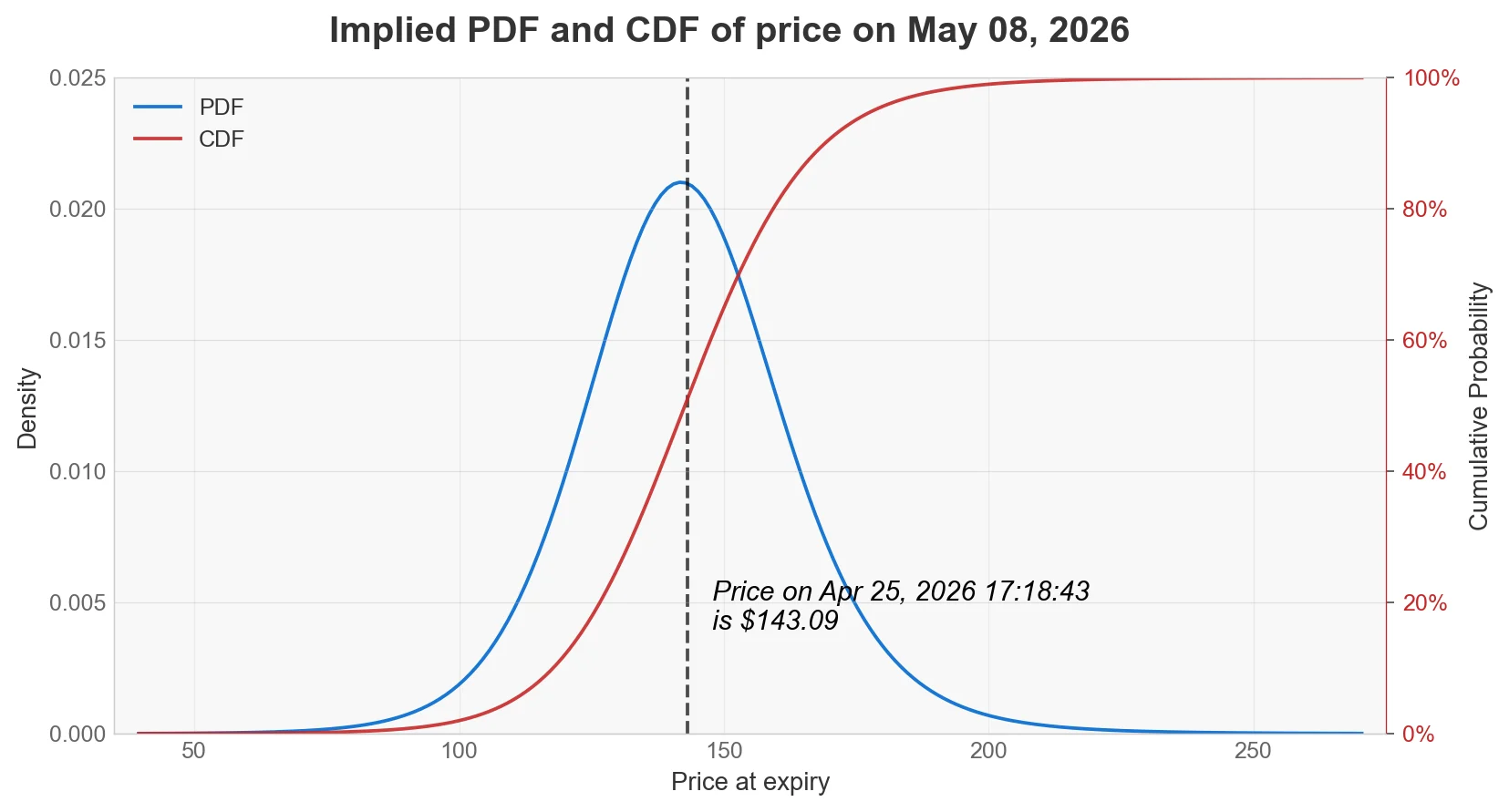
ProbCurve.from_chain requires a chain with a single expiry. If your DataFrame contains multiple expiry dates, OIPD raises a ValueError and asks you to use ProbSurface.from_chain instead.