> ## Documentation Index
> Fetch the complete documentation index at: https://docs.open-lemma.com/llms.txt
> Use this file to discover all available pages before exploring further.
# Quickstart
> Fetch a live options chain, fit a ProbCurve, and query market-implied tail probabilities, quantiles, and distributional moments in five steps.
This guide walks you through a complete end-to-end example: fetching a live options chain for a publicly traded stock, building the required market inputs, fitting a `ProbCurve`, and querying the resulting risk-neutral probability distribution. By the end you will have a working script you can adapt to any ticker.
Install the library from PyPI. The standard install includes the built-in yfinance data connection used in this guide.
```bash theme={null}
pip install oipd
```
Import the modules you need, then use `sources.list_expiry_dates` to see every available expiry for your ticker. Pass one of those dates to `sources.fetch_chain` to download the options chain and a market snapshot at the moment of download.
```python theme={null}
import matplotlib.pyplot as plt
from oipd import MarketInputs, ProbCurve, sources
ticker = "PLTR" # specify the stock ticker
expiries = sources.list_expiry_dates(ticker) # list all available expiry dates
single_expiry = expiries[1] # pick the expiry you're interested in
# fetch_chain returns the options chain and a market snapshot
chain, snapshot = sources.fetch_chain(ticker, expiries=single_expiry)
```
`chain` contains the full options chain (calls and puts, strikes, bid/ask, open interest). `snapshot` captures the underlying price and the timestamp of the download — both of which you need in the next step.
`MarketInputs` bundles the three pieces of market context that OIPD needs to fit the model: the valuation date, the underlying price, and the risk-free rate. Pull the first two directly from the snapshot you just downloaded.
```python theme={null}
market = MarketInputs(
valuation_date=snapshot.asof, # timestamp of the data download
underlying_price=snapshot.underlying_price, # spot price at download time
risk_free_rate=0.04, # use a Treasury yield close to your expiry horizon
)
```
For `risk_free_rate`, use the US Treasury or Fed Funds yield whose maturity most closely matches the time to your chosen expiry date.
Pass `chain` and `market` to `ProbCurve.from_chain`. This single call fits the SVI implied volatility smile and derives the risk-neutral probability distribution in one step.
```python theme={null}
prob = ProbCurve.from_chain(chain, market)
```
The returned `prob` object is fully fitted and immediately queryable. No separate `.fit()` call is needed when using the `from_chain` factory.
Use the query methods on the fitted `ProbCurve` to extract the statistics you care about.
```python theme={null}
prob_below = prob.prob_below(100) # P(price < 100)
prob_above = prob.prob_above(120) # P(price >= 120)
q50 = prob.quantile(0.50) # median implied price
skew = prob.skew() # distributional skew
```
| Method | What it returns |
| --------------- | ---------------------------------------------------------- |
| `prob_below(k)` | Cumulative probability that the price is below strike `k` |
| `prob_above(k)` | Probability that the price is at or above strike `k` |
| `quantile(q)` | The price level at the `q`-th quantile of the distribution |
| `skew()` | Skewness of the fitted risk-neutral distribution |
Call `prob.plot()` to render the probability distribution as a chart. It returns a Matplotlib `Figure`, so you can save it or customise it with standard Matplotlib calls.
```python theme={null}
fig = prob.plot() # kind="both" by default; also accepts "pdf" or "cdf"
plt.show()
```
To save the chart instead:
```python theme={null}
fig = prob.plot()
fig.savefig("probcurve.png", dpi=160, bbox_inches="tight")
```
Example output:
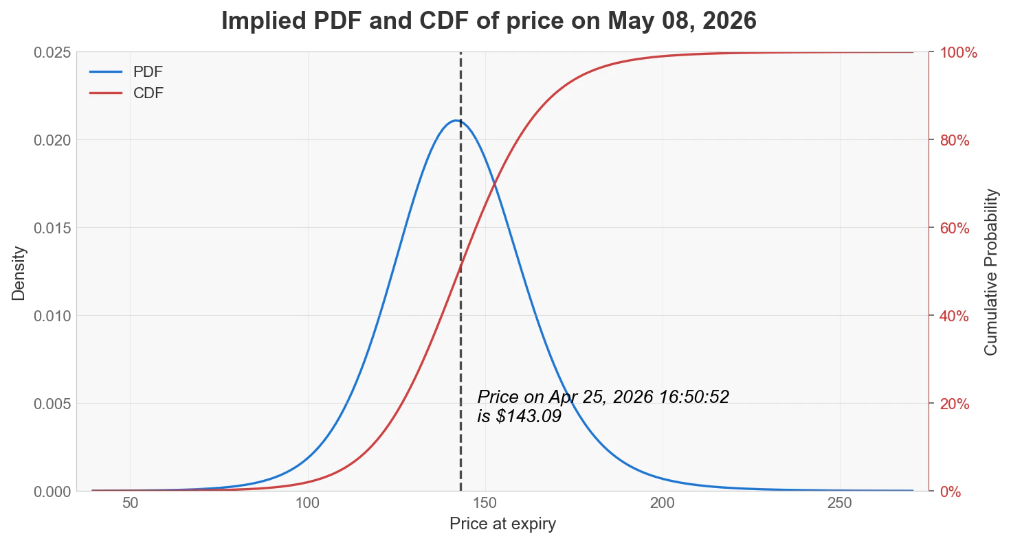 This example uses live option data, so your chart will differ as prices, expiries, and spreads update.
## Complete script
Here is the full example in one block, ready to copy and run:
```python theme={null}
import matplotlib.pyplot as plt
from oipd import MarketInputs, ProbCurve, sources
# 1. fetch data using the built-in yfinance connection
ticker = "PLTR"
expiries = sources.list_expiry_dates(ticker)
single_expiry = expiries[1]
chain, snapshot = sources.fetch_chain(ticker, expiries=single_expiry)
# 2. fill in market parameters
market = MarketInputs(
valuation_date=snapshot.asof,
underlying_price=snapshot.underlying_price,
risk_free_rate=0.04,
)
# 3. compute the probability distribution
prob = ProbCurve.from_chain(chain, market)
# 4. query and visualise
fig = prob.plot()
plt.show()
prob_below = prob.prob_below(100) # P(price < 100)
prob_above = prob.prob_above(120) # P(price >= 120)
q50 = prob.quantile(0.50) # median implied price
skew = prob.skew() # distributional skew
```
## Next steps
Fetch a multi-expiry chain with `sources.fetch_chain(..., horizon="12m")`, then pass it to `ProbSurface.from_chain`.
Work directly with `VolCurve` and `VolSurface` to evaluate implied vols, price options, and compute Greeks.
Load data from a CSV or Pandas DataFrame instead of yfinance for corporate or internal data environments.
Understand how OIPD surfaces data quality and model risk issues through structured diagnostics on every fitted object.
This example uses live option data, so your chart will differ as prices, expiries, and spreads update.
## Complete script
Here is the full example in one block, ready to copy and run:
```python theme={null}
import matplotlib.pyplot as plt
from oipd import MarketInputs, ProbCurve, sources
# 1. fetch data using the built-in yfinance connection
ticker = "PLTR"
expiries = sources.list_expiry_dates(ticker)
single_expiry = expiries[1]
chain, snapshot = sources.fetch_chain(ticker, expiries=single_expiry)
# 2. fill in market parameters
market = MarketInputs(
valuation_date=snapshot.asof,
underlying_price=snapshot.underlying_price,
risk_free_rate=0.04,
)
# 3. compute the probability distribution
prob = ProbCurve.from_chain(chain, market)
# 4. query and visualise
fig = prob.plot()
plt.show()
prob_below = prob.prob_below(100) # P(price < 100)
prob_above = prob.prob_above(120) # P(price >= 120)
q50 = prob.quantile(0.50) # median implied price
skew = prob.skew() # distributional skew
```
## Next steps
Fetch a multi-expiry chain with `sources.fetch_chain(..., horizon="12m")`, then pass it to `ProbSurface.from_chain`.
Work directly with `VolCurve` and `VolSurface` to evaluate implied vols, price options, and compute Greeks.
Load data from a CSV or Pandas DataFrame instead of yfinance for corporate or internal data environments.
Understand how OIPD surfaces data quality and model risk issues through structured diagnostics on every fitted object.