> ## Documentation Index
> Fetch the complete documentation index at: https://docs.open-lemma.com/llms.txt
> Use this file to discover all available pages before exploring further.
# Volatility surface
> Calibrate an implied volatility surface across many expiries, slice it within the fitted range, export long-format IV results, and convert to ProbSurface.
`VolSurface` extends single-expiry smile fitting to the term structure. It fits an SVI smile at each expiry in your chain, builds a total-variance interpolator between pillars, and exposes maturities within the fitted range as `VolCurve` slices. The guide below covers initialization, fitting, slicing, export, and conversion to a probability surface.
`VolSurface` takes the same constructor arguments as `VolCurve`. Configure the method and pricing engine once; the same settings apply to every expiry pillar.
```python theme={null}
from oipd import MarketInputs, ProbSurface, VolSurface, sources
vol_surface = VolSurface(method="svi", pricing_engine="black76")
```
Use `sources.fetch_chain` with a `horizon` argument to pull all expiries within your target window.
This example uses the built-in yfinance fetcher. For research or production work, your own vendor, broker, or exchange data will usually be cleaner. See [Data sources](/guides/data-sources) to load a CSV or DataFrame instead.
```python theme={null}
ticker = "PLTR"
chain_surface, snapshot_surface = sources.fetch_chain(ticker, horizon="12m")
surface_market = MarketInputs(
valuation_date=snapshot_surface.asof,
underlying_price=snapshot_surface.underlying_price,
risk_free_rate=0.04,
)
```
Call `vol_surface.fit(chain, market)`. The method requires at least two distinct expiries. By default it uses `failure_policy="skip_warn"`, which skips any expiry that fails to calibrate and records a `WorkflowWarning` rather than aborting the entire fit.
```python theme={null}
vol_surface.fit(chain_surface, surface_market)
```
**`failure_policy` options**
| Value | Behavior |
| ----------------------- | ----------------------------------------------------------- |
| `"skip_warn"` (default) | Skips failing expiries and continues fitting the surface. |
| `"raise"` | Raises a `CalculationError` on the first expiry that fails. |
**`horizon` filtering**
Pass `horizon` directly to `fit` to discard expiries beyond a cutoff, even if your chain already contains them:
```python theme={null}
vol_surface.fit(chain_surface, surface_market, horizon="6m")
```
Accepted formats: `"30d"`, `"6m"`, `"1y"`, or an explicit future date string or `datetime.date`.
`vol_surface.expiries` returns a sorted tuple of `pd.Timestamp` objects for every successfully fitted pillar. `vol_surface.slice(expiry)` returns a `VolCurve` at that maturity.
```python theme={null}
print(vol_surface.expiries) # (Timestamp(...), ...)
# Exact pillar — returns the original parametric curve
curve = vol_surface.slice(vol_surface.expiries[0])
print(curve.atm_vol)
print(curve.implied_vol([90, 100, 110]))
# Maturity between pillars — returns a synthetic interpolated VolCurve
midpoint = vol_surface.expiries[0] + (vol_surface.expiries[1] - vol_surface.expiries[0]) / 2
interp_curve = vol_surface.slice(midpoint)
print(interp_curve.atm_vol)
```
When you slice at a maturity that is not an exact fitted pillar, `VolSurface` derives a synthetic `VolCurve` from the total-variance interpolator. The interpolated curve supports `implied_vol`, `price`, `greeks`, and `implied_distribution` just like a directly fitted curve.
`iv_results` returns a long-format DataFrame spanning all fitted pillars. Supply `start`, `end`, and `step_days` to control the time grid.
```python theme={null}
# Default: daily grid from first to last fitted pillar
df = vol_surface.iv_results()
# Weekly grid over a custom range
df_range = vol_surface.iv_results(
start=vol_surface.expiries[0],
end=vol_surface.expiries[-1],
step_days=7,
)
# Pillar-only export
df_pillars = vol_surface.iv_results(step_days=None)
```
The DataFrame includes an `expiry` column. Set `include_observed=True` to add observed market bid/ask/mid IV columns from each pillar.
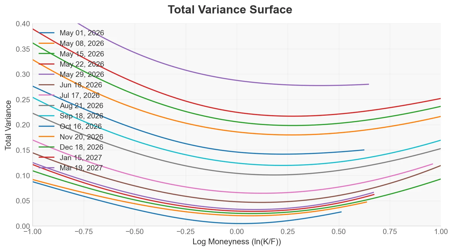
`plot` overlays the fitted smiles across the expiries that survived calibration. By default, it plots log-moneyness against total variance.
```python theme={null}
import matplotlib.pyplot as plt
fig = vol_surface.plot(xlim=(-1, 1), ylim=(0, 0.4))
plt.show()
```
Example output:
 Convert the fitted `VolSurface` to a `ProbSurface` with `implied_distribution()`. Use `ProbSurface.from_chain(...)` when you want OIPD to fit the volatility surface and derive probabilities in one step.
```python theme={null}
# From a fitted VolSurface
prob_surface = vol_surface.implied_distribution()
# Or as a one-liner from raw chain data
prob_surface = ProbSurface.from_chain(chain_surface, surface_market)
```
`VolSurface.fit` requires at least two unique expiries. A single-expiry chain raises a `CalculationError`. Use `VolCurve.fit` for single-expiry chains. Surface queries are limited to positive maturities up to the last fitted expiry.
Convert the fitted `VolSurface` to a `ProbSurface` with `implied_distribution()`. Use `ProbSurface.from_chain(...)` when you want OIPD to fit the volatility surface and derive probabilities in one step.
```python theme={null}
# From a fitted VolSurface
prob_surface = vol_surface.implied_distribution()
# Or as a one-liner from raw chain data
prob_surface = ProbSurface.from_chain(chain_surface, surface_market)
```
`VolSurface.fit` requires at least two unique expiries. A single-expiry chain raises a `CalculationError`. Use `VolCurve.fit` for single-expiry chains. Surface queries are limited to positive maturities up to the last fitted expiry.