> ## Documentation Index
> Fetch the complete documentation index at: https://docs.open-lemma.com/llms.txt
> Use this file to discover all available pages before exploring further.
# Volatility smile
> Configure and calibrate a single-expiry implied volatility smile, evaluate IVs, price options, compute Greeks, and export results with VolCurve.
`VolCurve` fits an implied volatility smile for a single option expiry. It follows a scikit-learn style workflow: configure an estimator, call `fit`, then evaluate the fitted object. The resulting smile lets you price options, compute Greeks, export IV data, and convert directly into a risk-neutral probability distribution. The steps below walk through the complete workflow.
Create a `VolCurve` with your chosen calibration algorithm and pricing engine. The default configuration uses SVI for the smile and Black-76 for IV inversion.
```python theme={null}
from oipd import MarketInputs, VolCurve, sources
vol = VolCurve(method="svi", pricing_engine="black76")
```
By default, use `pricing_engine="black76"`. OIPD infers the forward price from put-call parity, so the fitted forward already reflects the market's expected carry, including dividends. You do not need to enter dividends.
Download a single-expiry chain and populate `MarketInputs` from the vendor snapshot.
This example uses the built-in yfinance fetcher. For research or production work, your own vendor, broker, or exchange data will usually be cleaner. See [Data sources](/guides/data-sources) to load a CSV or DataFrame instead.
```python theme={null}
ticker = "PLTR"
expiries = sources.list_expiry_dates(ticker)
single_expiry = expiries[1]
chain, snapshot = sources.fetch_chain(ticker, expiries=single_expiry)
market = MarketInputs(
valuation_date=snapshot.asof,
underlying_price=snapshot.underlying_price,
risk_free_rate=0.04,
)
```
Call `vol.fit(chain, market)`. The method validates the chain, inverts IVs, calibrates the SVI parameters, and stores results on the instance.
```python theme={null}
vol.fit(chain, market)
```
Query IVs for any strike or array of strikes using either `implied_vol` or the callable shorthand.
```python theme={null}
import numpy as np
strikes = np.array([80, 90, 100, 110, 120])
ivs = vol.implied_vol(strikes) # returns np.ndarray
ivs = vol(strikes) # identical shorthand
atm = vol.atm_vol # IV where strike == forward price (float)
fwd = vol.forward_price # parity-implied forward price (float)
```
After fitting, `diagnostics` returns a dictionary of calibration metrics such as RMSE. `params` returns the raw SVI parameter set `{a, b, rho, m, sigma}`.
```python theme={null}
print(vol.diagnostics) # {"rmse": 0.0014, "status": "converged", ...}
print(vol.params) # {"a": ..., "b": ..., "rho": ..., "m": ..., "sigma": ...}
```
`vol.price` uses the fitted smile to value options at arbitrary strikes. `vol.greeks` returns a DataFrame with columns `strike`, `delta`, `gamma`, `vega`, `theta`, and `rho`.
```python theme={null}
prices = vol.price(strikes, call_or_put="call")
greeks_df = vol.greeks(strikes, call_or_put="call")
print(greeks_df)
# strike delta gamma vega theta rho
# 0 80.0 0.923 0.012 3.210 -0.041 0.172
# ...
```
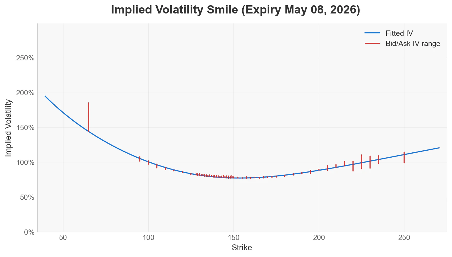
`iv_results` returns a DataFrame with the fitted smile curve alongside observed market bid/ask/mid IVs for quality-checking the calibration.
```python theme={null}
import matplotlib.pyplot as plt
smile_df = vol.iv_results(include_observed=True)
# columns: strike, fitted_iv, market_bid_iv, market_ask_iv, ...
fig = vol.plot(x_axis="strike", y_axis="iv")
plt.show()
```
Example output:
 Call `implied_distribution()` to derive a `ProbCurve` from the fitted smile. The returned object supports all probability queries described in the single-expiry probability guide.
```python theme={null}
prob = vol.implied_distribution()
print(prob.prob_below(100))
print(prob.quantile(0.50))
```
`VolCurve.fit` requires that the input chain contain exactly one expiry. If the DataFrame has multiple expiry dates, OIPD raises a `ValueError`. Use `VolSurface.fit` for multi-expiry chains.
Call `implied_distribution()` to derive a `ProbCurve` from the fitted smile. The returned object supports all probability queries described in the single-expiry probability guide.
```python theme={null}
prob = vol.implied_distribution()
print(prob.prob_below(100))
print(prob.quantile(0.50))
```
`VolCurve.fit` requires that the input chain contain exactly one expiry. If the DataFrame has multiple expiry dates, OIPD raises a `ValueError`. Use `VolSurface.fit` for multi-expiry chains.