> ## Documentation Index
> Fetch the complete documentation index at: https://docs.open-lemma.com/llms.txt
> Use this file to discover all available pages before exploring further.
# Probability surface
> Fit a risk-neutral probability surface over multiple expiries, query densities within the fitted range, and export a long-format results DataFrame.
`ProbSurface` extends single-expiry probability analysis to the full term structure. It calibrates a volatility smile at each listed expiry inside your horizon, interpolates between those pillars, and lets you query densities, CDFs, and quantiles within the calibrated range. The walkthrough below covers the complete workflow from data download to per-maturity slicing.
Pass `horizon` to `sources.fetch_chain` to automatically fetch every listed expiry within the requested window. The horizon string uses `w` for weeks, `m` for months, and `y` for years.
This example uses the built-in yfinance fetcher. For research or production work, your own vendor, broker, or exchange data will usually be cleaner. See [Data sources](/guides/data-sources) to load a CSV or DataFrame instead.
```python theme={null}
import matplotlib.pyplot as plt
from oipd import MarketInputs, ProbSurface, sources
ticker = "PLTR"
chain_surface, snapshot_surface = sources.fetch_chain(
ticker,
horizon="12m", # fetch all expiries within the next 12 months
)
```
The returned `chain_surface` is a single DataFrame containing all expiries. The `snapshot_surface` is a `VendorSnapshot` with `.asof`, `.underlying_price`, and `.vendor`.
Populate `MarketInputs` from the snapshot the same way you would for a single expiry.
```python theme={null}
surface_market = MarketInputs(
valuation_date=snapshot_surface.asof,
underlying_price=snapshot_surface.underlying_price,
risk_free_rate=0.04,
)
```
`ProbSurface.from_chain` fits SVI smiles at each expiry and wires up a total-variance interpolator for arbitrary-maturity queries.
```python theme={null}
surface = ProbSurface.from_chain(chain_surface, surface_market)
```
By default, the `failure_policy` is `"skip_warn"`, so individual expiries that fail to calibrate are skipped and recorded as `WorkflowWarning` events rather than aborting the whole fit. Pass `failure_policy="raise"` to make the first failure fatal.
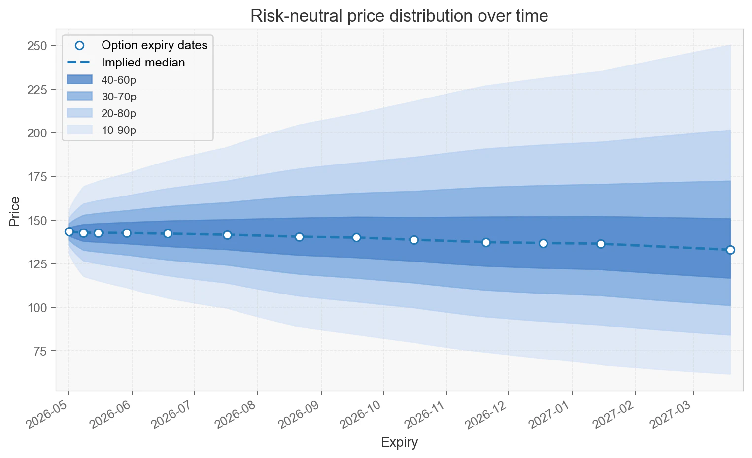
`plot_fan` draws risk-neutral quantile bands across all fitted maturities, giving you an at-a-glance view of how uncertainty spreads over time.
```python theme={null}
fig = surface.plot_fan()
plt.show()
```
Example output:
 The `t` parameter accepts a year-fraction float, including decimals, or a date-like value. Both forms work on `pdf`, `cdf`, and `quantile`, as long as the maturity falls within the fitted range.
```python theme={null}
# Year-fraction float
pdf_45d = surface.pdf(100, t=45/365) # density at K=100, 45 calendar days out
q50_45d = surface.quantile(0.50, t=45/365) # median price at 45 days
# Fractional days work too
t_2_5d = 2.5 / 365
cdf_2_5d = surface.cdf(100, t=t_2_5d)
# Date-like value
cdf_at_expiry = surface.cdf(100, t=surface.expiries[0])
```
When you pass a date that falls between two fitted expiry pillars, `ProbSurface` interpolates the volatility surface using a total-variance linear interpolator, then materializes the probability distribution at that synthetic maturity.
List the expiries that were successfully fitted with `surface.expiries`, then call `surface.slice(expiry)` to get a `ProbCurve` at any listed maturity. A sliced `ProbCurve` supports all the same query methods as one built directly from `ProbCurve.from_chain`.
```python theme={null}
print(surface.expiries) # tuple of pd.Timestamps
curve = surface.slice(surface.expiries[0])
print(curve.prob_below(100)) # P(price < 100)
print(curve.kurtosis()) # excess kurtosis
print(curve.quantile(0.50)) # median
```
`density_results` returns a long-format DataFrame with columns `expiry`, `price`, `pdf`, and `cdf`. By default it samples a daily grid between the first and last fitted pillar.
```python theme={null}
df = surface.density_results() # daily grid, all pillars
df_range = surface.density_results(
start=surface.expiries[0],
end=surface.expiries[-1],
step_days=7, # weekly grid
)
print(df_range.head())
```
Pass `step_days=None` to export only the exact fitted pillar expiries without interpolation.
`ProbSurface.from_chain` requires at least two expiries. If your chain contains only one expiry, OIPD raises a `CalculationError` and asks you to use `ProbCurve.from_chain` instead. Surface queries are limited to positive maturities up to the last fitted expiry.
The `t` parameter accepts a year-fraction float, including decimals, or a date-like value. Both forms work on `pdf`, `cdf`, and `quantile`, as long as the maturity falls within the fitted range.
```python theme={null}
# Year-fraction float
pdf_45d = surface.pdf(100, t=45/365) # density at K=100, 45 calendar days out
q50_45d = surface.quantile(0.50, t=45/365) # median price at 45 days
# Fractional days work too
t_2_5d = 2.5 / 365
cdf_2_5d = surface.cdf(100, t=t_2_5d)
# Date-like value
cdf_at_expiry = surface.cdf(100, t=surface.expiries[0])
```
When you pass a date that falls between two fitted expiry pillars, `ProbSurface` interpolates the volatility surface using a total-variance linear interpolator, then materializes the probability distribution at that synthetic maturity.
List the expiries that were successfully fitted with `surface.expiries`, then call `surface.slice(expiry)` to get a `ProbCurve` at any listed maturity. A sliced `ProbCurve` supports all the same query methods as one built directly from `ProbCurve.from_chain`.
```python theme={null}
print(surface.expiries) # tuple of pd.Timestamps
curve = surface.slice(surface.expiries[0])
print(curve.prob_below(100)) # P(price < 100)
print(curve.kurtosis()) # excess kurtosis
print(curve.quantile(0.50)) # median
```
`density_results` returns a long-format DataFrame with columns `expiry`, `price`, `pdf`, and `cdf`. By default it samples a daily grid between the first and last fitted pillar.
```python theme={null}
df = surface.density_results() # daily grid, all pillars
df_range = surface.density_results(
start=surface.expiries[0],
end=surface.expiries[-1],
step_days=7, # weekly grid
)
print(df_range.head())
```
Pass `step_days=None` to export only the exact fitted pillar expiries without interpolation.
`ProbSurface.from_chain` requires at least two expiries. If your chain contains only one expiry, OIPD raises a `CalculationError` and asks you to use `ProbCurve.from_chain` instead. Surface queries are limited to positive maturities up to the last fitted expiry.