> ## Documentation Index
> Fetch the complete documentation index at: https://docs.open-lemma.com/llms.txt
> Use this file to discover all available pages before exploring further.
# Probability curve
> Step-by-step guide to fitting a risk-neutral probability distribution on a single option expiry date and querying prices, quantiles, and moments.
Option prices imply a risk-neutral distribution over future prices. `ProbCurve` extracts that distribution from a single-expiry option chain by fitting an SVI volatility smile and converting it into probabilities. The walkthrough below takes you from data download to distributional statistics in five steps.
Start by fetching the available expiry dates for your ticker. `sources.list_expiry_dates` calls the built-in yfinance connection and returns dates as `YYYY-MM-DD` strings.
```python theme={null}
from oipd import MarketInputs, ProbCurve, sources
ticker = "PLTR"
expiries = sources.list_expiry_dates(ticker) # list of "YYYY-MM-DD" strings
single_expiry = expiries[1] # pick the expiry you want
print(single_expiry) # one of the returned expiry dates
```
Pass the selected expiry to `sources.fetch_chain`. It returns two objects: a normalized `chain` DataFrame and a `VendorSnapshot` that records the underlying price and download timestamp.
This example uses the built-in yfinance fetcher. For research or production work, your own vendor, broker, or exchange data will usually be cleaner. See [Data sources](/guides/data-sources) to load a CSV or DataFrame instead.
```python theme={null}
chain, snapshot = sources.fetch_chain(ticker, expiries=single_expiry)
# snapshot fields you will use:
# snapshot.asof — datetime of the data pull
# snapshot.underlying_price — spot price at download time
# snapshot.vendor — "yfinance"
```
`MarketInputs` bundles the market context needed for calibration. Use the snapshot fields to avoid mis-dating your inputs.
```python theme={null}
market = MarketInputs(
valuation_date=snapshot.asof, # datetime of the data pull
underlying_price=snapshot.underlying_price, # spot price at download time
risk_free_rate=0.04, # annualized risk-free rate
)
```
Use a US Treasury yield whose maturity is closest to your target expiry date. The default `risk_free_rate_mode` is `"annualized"` (simple ACT/365). Pass `risk_free_rate_mode="continuous"` if your rate source is continuously compounded.
`ProbCurve.from_chain` fits an SVI volatility smile and derives the risk-neutral distribution in one call.
```python theme={null}
prob = ProbCurve.from_chain(chain, market)
```
By default the library repairs minor CDF monotonicity issues and records a `ModelRiskWarning`. Use `cdf_violation_policy="raise"` if you want strict violations to propagate as errors instead.
Once fitted, `ProbCurve` exposes probability queries, distributional moments, a plot method, and a DataFrame export.
**Probability queries**
```python theme={null}
prob_below = prob.prob_below(100) # P(price < 100)
prob_above = prob.prob_above(120) # P(price >= 120)
prob_range = prob.prob_between(90, 110) # P(90 <= price < 110)
```
**Quantiles and moments**
```python theme={null}
q50 = prob.quantile(0.50) # median implied price
mean = prob.mean() # expected price E[S]
skew = prob.skew() # 3rd standardized moment
kurt = prob.kurtosis() # excess kurtosis (0 = normal)
```
**Visualization**
```python theme={null}
import matplotlib.pyplot as plt
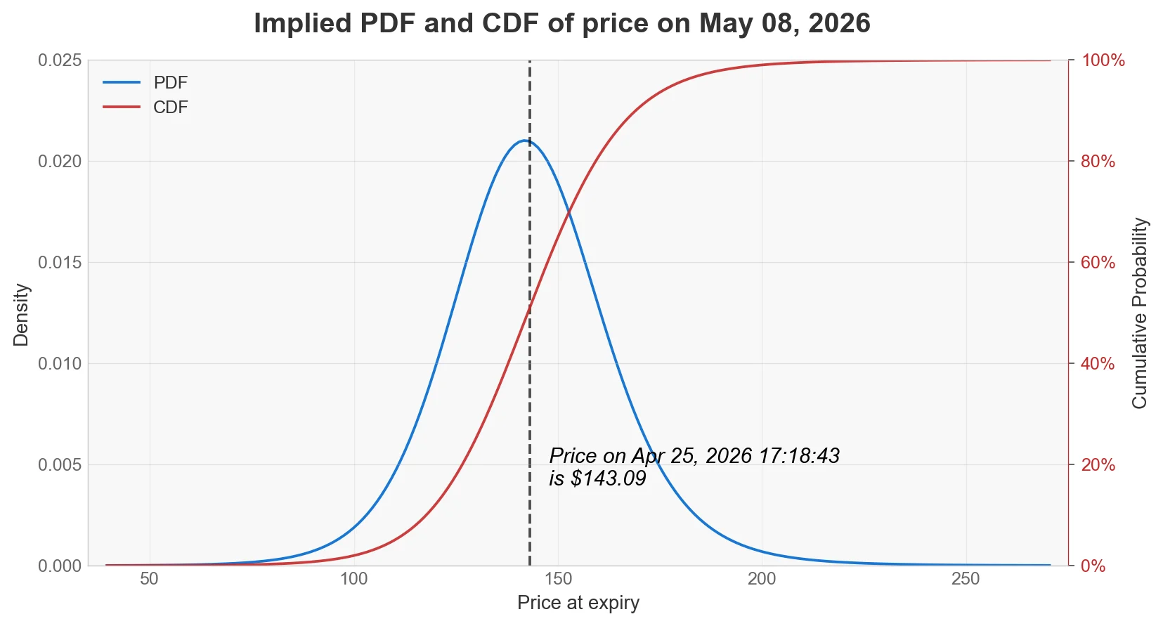
fig = prob.plot(kind="both") # overlays PDF and CDF; also "pdf" or "cdf"
plt.show()
```
Example output:
 **Export to DataFrame**
`density_results()` returns a `DataFrame` with columns `price`, `pdf`, and `cdf`.
```python theme={null}
df = prob.density_results()
print(df.head())
```
`ProbCurve.from_chain` requires a chain with a single expiry. If your DataFrame contains multiple expiry dates, OIPD raises a `ValueError` and asks you to use `ProbSurface.from_chain` instead.
**Export to DataFrame**
`density_results()` returns a `DataFrame` with columns `price`, `pdf`, and `cdf`.
```python theme={null}
df = prob.density_results()
print(df.head())
```
`ProbCurve.from_chain` requires a chain with a single expiry. If your DataFrame contains multiple expiry dates, OIPD raises a `ValueError` and asks you to use `ProbSurface.from_chain` instead.